Dalyander, P. Soupy , 2014, GMEX_95th_perc: The 95th percentile of bottom shear stress for the Gulf of Mexico, May 2010 to May 2011 (Geographic, WGS 84): Online Database, U.S. Geological Survey, Coastal and Marine Geology Program, Woods Hole Coastal and Marine Science Center, Woods Hole, MA.This is part of the following larger work.Online Links:
Dalyander, P.S., Butman, B., Sherwood, C.R., and Signell, R.P., 2012, U.S. Geological Survey Sea Floor Stress and Sediment Mobility Database: Online Database, U.S. Geological Survey, Coastal and Marine Geology Program, Woods Hole Coastal and Marine Science Center, Woods Hole, MA.Online Links:
Horizontal positions are specified in geographic coordinates, that is, latitude and longitude. Latitudes are given to the nearest 0.000001. Longitudes are given to the nearest 0.000001. Latitude and longitude values are specified in Decimal degrees.
The horizontal datum used is D_WGS_1984.
The ellipsoid used is WGS_1984.
The semi-major axis of the ellipsoid used is 6378137.000000.
The flattening of the ellipsoid used is 1/298.257224.
Sequential unique whole numbers that are automatically generated.
Coordinates defining the features.
| Range of values | |
|---|---|
| Minimum: | 0.0122 |
| Maximum: | 1.5296 |
| Units: | Pa |
| Resolution: | 0.0001 |
| Range of values | |
|---|---|
| Minimum: | 0.0130 |
| Maximum: | 2.6280 |
| Units: | Pa |
| Resolution: | 0.0001 |
| Range of values | |
|---|---|
| Minimum: | 0.0080 |
| Maximum: | 1.7294 |
| Units: | Pa |
| Resolution: | 0.0001 |
| Range of values | |
|---|---|
| Minimum: | 0.0088 |
| Maximum: | 1.6574 |
| Units: | Pa |
| Resolution: | 0.0001 |
| Range of values | |
|---|---|
| Minimum: | 0.0011 |
| Maximum: | 1.3600 |
| Units: | Pa |
| Resolution: | 0.0001 |
(727) 502-8000 x8124 (voice)
(727) 502-8001 (FAX)
sdalyander@usgs.gov
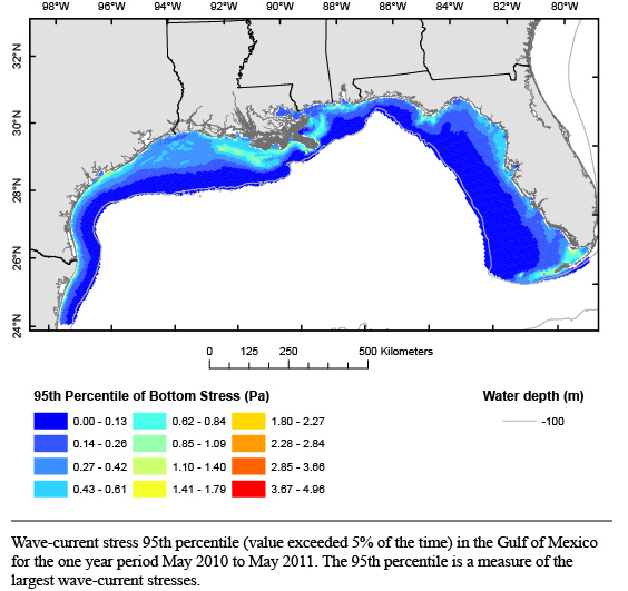
This GIS layer contains an estimate of the 95th percentile of bottom shear stress for the Gulf of Mexico. This output is based on statistical characterization of numerical model estimates of wave and circulation patterns over an approximately one year time frame. This data layer is primarily intended to show the overall distribution of the highest stress values on large spatial scales, and should be used qualitatively. Intended users include scientific researchers and the coastal and marine spatial planning community.
NOAA National Centers for Environmental Prediction (NCEP), 20110601, NOAA/NCEP Global Forecast System (GFS) Atmospheric Model: NOAA National Centers for Environmental Prediction, Camp Springs, MD.Online Links:
NOAA National Centers for Environmental Prediction (NCEP), 20110601, NOAA/NCEP North American Mesoscale (NAM) Atmospheric Model: NOAA National Centers for Environmental Prediction, Camp Springs, MD.Online Links:
North Carolina State University, 2012, South Atlantic Bight and Gulf of Mexico Circulation Nowcast/Forecast (SABGOM N/F): North Carolina State University, Raleigh, North Carolina.Online Links:
The SABGOM hydrodynamic model (<http://omgsrv1.meas.ncsu.edu:8080/ocean-circulation/>) is operated by North Carolina State University as a quasi-operational nowcast/forecast system in the Southeast Coastal Ocean Observing Regional Association (SECOORA, <http://secoora.org/>), part of the U.S. Integrated Ocean Observing System (<http://www.ioos.noaa.gov/>). The underlying circulation model is the Regional Ocean Modeling System (ROMS; <http://www.myroms.org>), a finite-difference, hydrostatic, primitive equation ocean model that solves for the free surface elevation and three dimensional flow patterns, temperature, and salinity.
The SABGOM configuration of ROMS has 5 km horizontal resolution and 36 layers in vertical terrain-following coordinates. Ocean open boundary values are from a global forecast that uses the HYbrid Coordinate Ocean Model (HyCOM) with assimilation of satellite and in situ data with the Navy Coupled Ocean Data Assimilation (NCODA) system. Tidal harmonic boundary variability is determined from a regional tidal model.
The datafiles for the time period used in this analysis were acquired directly from Dr. Ruoying He of NCSU.
NOAA National Centers for Environmental Prediction (NCEP, 20110601, NOAA/NWS/NCEP Global Wavewatch III Operational Wave Forecast: NOAA National Centers for Environmental Prediction, Camp Springs, MD.Online Links:
Person who carried out this activity:
(727) 502-8000 x8124 (voice)
(727) 502-8001 (FAX)
sdalyander@usgs.gov
Data sources produced in this process:
Full spectra boundary conditions at each model ocean boundary point are interpolated from the output of the regional 10' Wavewatch III model, updated every hour. Wind forcing was provided at 3-hour resolution from the NOAA North American Mesoscale (NAM) model (12 km resolution) over its domain, with forcing at the most offshore portions of the grid (outside the NAM grid) provided by the NOAA Global Forecasting System (GFS) model at 0.5 degree resolution. The SWAN directional resolution was 6 degrees (60 bins), determined via sensitivity analysis as the coarsest (and hence least computationally expensive) resolution that does not result in the "Garden-Sprinkler Effect" (GSE), wherein swell traveling over large distances inaccurately disintegrates into non-continuous wave fields as a result of frequency and directional discretization. The minimum frequency bin should be set to a value less than 0.7 times the lowest expected peak frequency and the maximum frequency bin should be set at least 2.5-3 times the highest expected peak frequency expected. In order to determine appropriate values, the peak periods from 43 NDBC buoys throughout the wave model domain were analyzed (when available) over the one year period of the study, yielding 297,533 hourly observations. The 99th and 1st percentiles of peak period were 15 s and 3 s, corresponding to frequencies of 0.07 Hz and 0.33 Hz, noting that these values may be biased by buoy limits of detection at high and low frequencies. The frequency range was therefore specified as 0.04-1 Hz. SWAN was allowed to internally determine the frequency resolution as one tenth of each frequency bin for best performance of the discrete interaction approximation (DIA) method of nonlinear 4-wave interactions, resulting in 34 frequency bins. Bottom friction calculations used the Madsen formulation with a uniform roughness length scale of 0.05 m. This value was selected for the best comparison of model output and buoy observations within the domain, and does not correspond to physical roughness values or the bottom roughness used in stress calculations. Wind generation and whitecapping parameterizations follow the modified Komen approach prescribed by Rogers et al. (2003), which reduces inaccurate attenuation of swell energy by whitecapping. Wave model outputs of bottom orbital velocity, bottom representative period, and bottom wave direction were output hourly and interpolated onto the SABGOM model grid.
The same person that conducted this processing step conducted each subsequent processing step.
References:
Rogers, W.E., Hwang, P.A., Wang, D.W., 2003. Investigation of Wave Growth and Decay in the SWAN Model: Three Regional-Scale Applications. J. Phys. Oceanogr. 33, 366-389.
Person who carried out this activity:
(727) 502-8000 x8124 (voice)
(727) 502-8001 (FAX)
sdalyander@usgs.gov
Data sources produced in this process:
Wave direction, bottom orbital velocities, and bottom periods are calculated internally by the wave model. Near-bed current magnitude and direction are taken from the hydrodynamic model, with the reference height taken as the distance from the cell vertical midpoint to the seabed. GM requires that the current velocity be taken above the wave boundary layer (WBL) but within the log-profile current velocity layer. If the thickness of the WBL calculated using GM exceeds of one or more of the deepest grid cells, the current estimate and associated reference height are used from the deepest grid cell at each location where the reference height exceeds the width of the WBL. An estimate must be used for the maximum reference height where the log-profile velocity layer assumption is valid. As discussed in Grant and Madsen (1986), the thickness of the log-profile layer based on laboratory experiments is approximately 10% of the current boundary layer thickness (Clauser, 1956). Because tidal currents, storm currents, and mean flow have a boundary layer thickness on the order of magnitude 10's of meters (Goud, 1987), a maximum value for reference height is set as 5 m. The GM bottom boundary layer model also requires a value for bottom roughness; a uniform value of 0.005 m is used throughout the domain.
References:
Clauser, F.H., 1956. The turbulent boundary layer. Adv. Appl. Mech. 4, 1-51.
Madsen, O.S., 1994. Spectral wave-current bottom boundary layer flows, Proceedings 24th Conf. Coastal Eng., pp. 384-398.
Glenn, S.M., 1983. A Continental Shelf Bottom Boundary Layer Model: The Effects of Waves, Currents, and a Moveable Bed. Dissertation, Massachusetts Institute of Technology and Woods Hole Oceanographic Institution, Cambridge, MA, 237 pp.
Glenn, S.M., Grant, W.D., 1987. A suspended sediment stratification correction for combined wave and current flows. J. Geophys. Res. 92, 8244-8264.
Goud, M.R., 1987. Prediction of Continental Shelf Sediment Transport Using a Theoretical Model of the Wave-Current Boundary Layer. Dissertation, Massachusetts Institute of Technology and Woods Hole Oceanographic Institution, Cambridge, MA, 211 pp.
Grant, W.D., Madsen, O.S., 1986. The continental-shelf bottom boundary-layer. Annu. Rev. Fluid Mech. 18, 265-305.
Grant, W.D., Madsen, O.S., 1982. Movable bed roughness in unsteady oscillatory flow. J. Geophys. Res. 87, 469-481.
Grant, W.D., Madsen, O.S., 1979. Combined wave and current interaction with a rough bottom J. Geophys. Res. 84, 1797-1808.
Madsen, O.S., 1994. Spectral wave-current bottom boundary layer flows, Proceedings 24th Conf. Coastal Eng., pp. 384-398.
Madsen, O.S., Poon, Y., Graber, H.C., 1988. Spectral wave attenuation by bottom friction: theory, Proceedings 21st Int. Conf. Coast. Eng., pp. 492-504.
Data sources used in this process:
Data sources produced in this process:
Data sources used in this process:
Data sources produced in this process:
Data sources used in this process:
U.S. Geological Survey, 2012, Documentation of the U.S. Geological Survey Sea Floor Stress and Sediment Mobility Database: Open-File Report 2012-1137, U.S. Geological Survey, Reston, VA.Online Links:
Each attribute in this data layer covers a specific time period of interest. The attributes include winter (December - February), spring (March - May), summer (June - August), fall (September - November), and the entire year. Each of these attributes was calculated from model output spanning May, 2010 to May, 2011. Statistical values will vary somewhat if calculated from model parameters covering a different time period, or if a different numerical model is used to estimate the time-series of waves and circulation used in calculating the time-series of bottom shear stress.
Numerical models are used in the generation of time-series of bottom shear stress used in creating this data layer. Because the overall horizontal accuracy of the data set depends on the accuracy of the model, the underlying bathymetry, and forcing values used, and so forth, the spatial accuracy of this data layer cannot be meaningfully quantified. These maps are intended to provide a qualitative and relative regional assessment of bottom shear stress at the approximately 5 km resolution displayed; users are advised not to use the data set to estimate shear stress quantitatively at any specific geographic location.
All model output values were used in the calculation of this statistic. The statistic was calculated for the date range of May 2010 to May 2011, and would potentially vary somewhat if performed on a different time period. The underlying time-series of bottom shear stress was calculated from wave and current estimates generated with numerical models, and would vary if different models are used or if different model inputs (such as bathymetry or forcing winds) or parameterizations were chosen.
No duplicate features are present. All polygons are closed, and all lines intersect where intended. No undershoots or overshoots are present.
Are there legal restrictions on access or use of the data?
- Access_Constraints: None
- Use_Constraints:
- Public domain data from the U.S. Government are freely redistributable with proper metadata and source attribution. Please recognize the U.S. Geological Survey as the originator of the dataset.
(727) 502-8000 x8124 (voice)
(727) 502-8001 (FAX)
sdalyander@usgs.gov
Downloadable Data: Sea Floor Stress and Sediment Mobility Database, 95th percentile of bottom shear stress for the Gulf of Mexico (GMEX_95th_perc)
Neither the U.S. Government, the Department of the Interior, nor the USGS, nor any of their employees, contractors, or subcontractors, make any warranty, express or implied, nor assume any legal liability or responsibility for the accuracy, completeness, or usefulness of any information, apparatus, product, or process disclosed, nor represent that its use would not infringe on privately owned rights. The act of distribution shall not constitute any such warranty, and no responsibility is assumed by the USGS in the use of these data or related materials.Any use of trade, product, or firm names is for descriptive purposes only and does not imply endorsement by the U.S. Government.
| Data format: | WinZip archive file containing the shapefile components. The WinZip file also includes FGDC compliant metadata. in format Shapefile (version ArcGIS 9.3) Esri shapefile Size: 1.164 |
|---|---|
| Network links: |
<http://woodshole.er.usgs.gov/project-pages/mobility/gmex.html> <http://woodshole.er.usgs.gov/project-pages/mobility/ArcData/GMEX_95th_perc.zip> <http://woodshole.er.usgs.gov/project-pages/mobility/index.html> |
These data are available in Esri shapefile format. The user must have ArcGIS or ArcView 3.0 or greater software to read and process the data file. In lieu of ArcView or ArcGIS, the user may utilize another GIS application package capable of importing the data. A free data viewer, ArcExplorer, capable of displaying the data is available from Esri at www.esri.com.
(727) 502-8000 x8124 (voice)
(727) 502-8001 (FAX)
sdalyander@usgs.gov