
USGS Development Version of ROMS
Solution to Test Case 2: Estuary
|
Model: ROMS v2.0 Date: September 3, 2002 Modeller: John C. Warner (jcwarner@usgs.gov), USGS Woods Hole Field Center 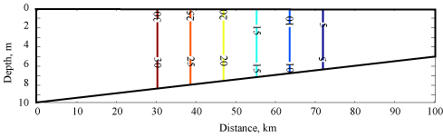
Figure 1. Initial salinity distribution for estuary simulations Model was initialized with a constant longitudinal salinity field as shown in Figure 1. Simulations were the calculated for 20 tidal cycles (10 days), after which time a quasi-steady state had been reached. Figure 2 shows the resulting salinity fields for 4 different closure methods near the end of 20 tidal cycles. The 4 different closures are: MY25, Generic Length Scale (GLS) as KKL, GLS as KE, and GLS as KW88. The MY25 closure is computed based on the classical scheme of Mellor/Yamada (1982), and the GLS closures are computed with the method of Umlauf and Burchard (2002 submitted). The main difference is in the length scale limitations. For the MY25 method, the length scale is only limited in the calculation of the stability functions, whereas for the GLS method the length scale is limited in the production, wall proximity function, and the stability functions. 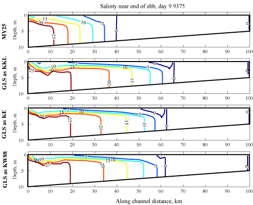
Figure 2. Salinity distribution after 9.9 days for the estuary simulations. Suspended sediment results (figure 3) are very dependent on the bottom stresses and vertical mixing processes. For these simulations, a thin layer of sediment was placed on the bed at time = 10 days. Sediment parameters were selected to allow rapid erosion. Upstream riverine flow will transport the sediment downstream and the estuarine circulation creates a turbidity maximum at the limit of salt intrusion. For the MY25 closure, this limit is near x = 35 km, while for the KE and KW simulations, a near bottom turbidity maximum is located near x = 50 km. For the KKL simulation, the turbidity maximum is further upstream, near x = 60 km. 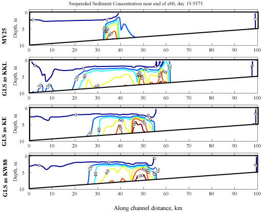
Figure 3. Suspended sediment concentration distribution after 9.9 days for the estuary simulations. |

