Introduction Time-series photographs of the sea floor were obtained from an instrumented tripod deployed in western Massachusetts Bay at LT-A (42° 22.6' N, 70° 47.0' W, 32 m water depth, fig. 1) from December 1989 through September 2005. The photographs provide time-series observations of physical changes of the sea floor, near-bottom water turbidity, and life on the sea floor. Two reports present these photographs in digital form (table 1) and chronological order. U.S. Geological Survey Data Series 265 (Butman and others, 2008a) contains the photographs obtained from December 1989 to October 1996. This report, U.S. Geological Survey Data Series 266 (Butman and others, 2008b), contains photographs obtained from October 1996 through September 2005. The photographs are published in separate reports because the data are too large for distribution on a single DVD. This report also contains photographs that were published previously in an uncompressed format (Butman and others 2004a, b, and c, table 1); they have been compressed and included in this publication so that all of the photographs are available in the same format. The photographs, obtained every 4 or every 6 hours, are presented as individual photographs (in .png format, each accessible through a page of thumbnails) and as a movie (in .avi format). The time-series photographs taken at LT-A were collected as part of a U.S. Geological Survey (USGS) study to understand the transport and fate of sediments and associated contaminants in Massachusetts Bay and Cape Cod Bay (Bothner and Butman, 2007). This long-term study was carried out by the USGS in partnership with the Massachusetts Water Resources Authority (MWRA) (http://www.mwra.state.ma.us/) and with logistical support from the U.S. Coast Guard (USCG). Long-term oceanographic observations help to identify the processes causing bottom sediment resuspension and transport and provide data for developing and testing numerical models. The observations document seasonal and interannual changes in currents, hydrography, and suspended-matter concentration, and the importance of infrequent catastrophic events, such as major storms, in sediment resuspension and transport. LT-A is approximately 1 km south of the ocean outfall that began discharging treated sewage effluent from the Boston metropolitan area into Massachusetts Bay in September 2000. See Butman and others (2004) and Butman, Bothner and others (2007) for a description of the oceanographic measurements at LT-A. See Butman, Warner, and others (2007) and Warner and others (2007) for discussion of sediment transport in Massachusetts Bay. Instrumentation The time-lapse bottom photographs were obtained by means of a Benthos 35-mm camera mounted on a tripod frame that rests on the sea floor (figs. 2 and 3). The camera (fig. 4) was mounted about 1.5 m above the sea floor and aimed downwards; a strobe (fig. 5) illuminated the sea floor from one side of the photograph. The field of view of the camera is 54 degrees, resulting in a photograph area on the sea floor measuring approximately 1.5 m x 1 m. A compass and vane (fig. 6) mounted in the field of view of the camera show the instantaneous direction of current flow and the scale and orientation of the photographs. The photographs were taken on Kodak 35-mm Ektachrome Professional Film (E200, a daylight-balanced 200-speed color transparency film, 100-ft roll, about 700 photographs/roll). The Benthos camera places the photographs in a nonstandard format along the long axis of the film. This allows a photograph of the sea floor larger than what would be possible if the photograph were placed across the film in a standard 35-mm format. The film is advanced using an O-ring drive; the loose drive and drive-motor inertia cause the distance between frames to vary slightly with each photograph. The unevenly spaced photographs required alignment to view them as a time-series movie without jitter. The camera and strobe were controlled by a timer set to obtain an photograph every 4 or 6 hours, depending on the deployment. The time of each photograph differs from a uniform spacing by a few minutes because of drift in this analog controller. A digital light emitting diode (LED) clock, separate from the controller, places the hour, minute, second, and day on each photograph. The day counter on the LED clock counts to 31 and then resets back to 1. The time on the LED typically differed from true time by a few minutes at the end of the deployment and thus is assumed to provide a reasonably accurate time for each photograph. Instrumentation mounted on the same tripod frame measured current speed and direction, temperature, light transmission, conductivity, and pressure every 3.75 minutes (Butman and others, 2004). Light transmission is a measure of water clarity and was converted to beam attenuation (attenuation = - 4ln(percent transmission over 0.25 m)). Current was sampled, typically at 2 Hz, and vector-averaged to provide a mean current every 3.75 minutes. Pressure was also sampled at 2 Hz; the standard deviation of pressure (called PSDEV) was computed every 3.75 minutes as a measure of wave-induced fluctuations at the sea floor. Plots of these data are included in the .avi movies. USGS began to develop a new digital bottom camera system in 2004 to replace the aging Benthos film systems. A timing interface was developed to control a Konica Minolta A2 camera; the system was housed in a PVC pressure case with 100 m depth capability (fig. 7). Two deployments were made to test this new camera system in 2005. The picture interval was every 8 hours. Pictures of the sea floor obtained in these deployments are included in this report as single images. Instrument Deployments During the USGS study, instrumented tripods were deployed and recovered at LT-A three times each year, typically in February, May or June, and September. This report presents photographs obtained during 19 deployments that took place during the period October 1996 through September 2005. The deployments are identified by a 3-digit USGS mooring number that is assigned sequentially to all instrument deployments (table 2). The camera on tripods 632 and 708 failed to operate. Because of camera and strobe failures, systems were not available to be deployed on tripods 611, 645, 683, 697, and 756 (table 1). Each tripod was located near the USCG Boston approach B Buoy (National Ocean Service, 1997) on the southern flank of a ridge in water about 32 m deep (fig. 8). This location was selected for long-term observations because the USCG buoy marked the site and provided some physical protection from other marine activities. Table 2. USGS mooring number, date and location of time-series photographs contained in this Data Series report. Mooring Number Start/Stop Date Latitude (N) Longitude (W) Water Depth (m) 480 October 1996 February 1997 42 22.74 70 46.84 31 495 February 17, 1997 June 10, 1997 42 22.63 70 47.07 31 501 June 10, 1997 September 23, 1997 42 22.63 70 47.07 31 507 September 23, 1997 November 12, 1997 42 22.64 70 47.07 31 516 February 10, 1998 June 10, 1998 42 22.62 70 47.08 31 530 June 17, 1998 September 30, 1998 42 22.62 70 47.08 31 540 September 30, 1999 February 8, 1999 42 22.64 70 47.09 31 552 February 10, 1999 May 7, 1999 42 22.64 70 47.07 31 569 May 11, 1999 September 15, 1999 42 22.68 70 47.09 33 591 September 26, 1999 December 10, 1999 42 22.68 70 47.09 31 625 May 13, 2000 September 11, 2000 42 22.69 70 47.09 30 638 February 14, 2001 May 24, 2001 42 22.68 70 47.09 31 665 October 23, 2001 February 6, 2002 42 22.68 70 47.09 30 690 May 21, 2002 September 23, 2002 42 22.67 70 47.10 31 717 September 24, 2003 February 1, 2004 42 22.68 70 46.09 31 767 May 19, 2004 July 17, 2004 42 22.68 70 46.09 31 775 September 22, 2004 January 27, 2005 42 22.72 70 46.84 31 777 February 9, 2005 May 18, 2005 42 22.72 70 46.85 32 786 May 18, 2005 September 28, 2005 42 22.72 70 46.85 33 Digitizing the Films Each photograph on the 35-mm film was digitized as an image in tif format at a resolution of 1920 by 1080 pixels at the Woods Hole Oceanographic Institution (WHOI) using a special film transport mechanism and aligned using Combustion 4.0 (http://dv411.com/combustion4.html) and Shake 5.0 (http://www.apple.com/shake/) software. The photographs were reduced to 600 by 337 pixels using PolyView (www.polybytes.com) and compressed to 256-color .png images using IrfanView (http://www.irfanview.com/), reducing the photograph size by about a factor of 6. This photograph size and compression provide reasonable resolution and manageable size for publication. Some of time-series photographs were previously published in an uncompressed version (Butman and others 2004a, 2004b, 2004c, table 1); these movies and images have been compressed and are included in this publication so that all of the time-series are available in the smaller file size. The full resolution digital photographs and the original 35-mm films are archived at the USGS Woods Hole Science Center. This publication includes all of the photographs in this archive, even some of poor quality. Creating the Time-Lapse Movies Time-lapse movies were created from the digitized photographs using MATLAB software (www.mathworks.com). The photographs collected at approximately 4-hour intervals (deployments 338 through 383) or 6-hour intervals (deployments 389 through 775) were distributed at an even interval between the start and stop time of the photographic record, as determined from the LED clock. The LED clock time was checked for consistency with camera on times and tripod deployment and recovery times as recorded in field logs. During the deployment, the camera controller occasionally malfunctioned; in order to provide an equally spaced time-series, missed photographs were filled with blanks and multiple photographs were deleted. The LED clock was sometimes set ahead of the true date to maximize the amount of time during a deployment that the clock would display the correct day (for example, the day counter of the LED clock was set three days ahead if the tripod was deployed in February to have the counter be correct during March and April). These offsets are corrected in the time displayed below the data panel, and in the times in table 4 . The data plots shown with the photographs were made with MATLAB. The movies were compressed with the Microsoft Video 1 codec using VideoMach (http://www.gromada.com/). This reduced the .avi file size by a factor of about 6. Viewing Movies and Photographs The movies may be viewed using a movie player such as Imagen (available free at http://www.gromada.com/imagen.html), QuickTime (available free at http://www.apple.com/quicktime/download/) or Windows Media Player. Click on Movie in table 3 to open or download the movie, or navigate to the .avi file on the DVD (located in directories labeled TRIPODNNN, where NNN is the mooring number) and open with a movie player. See below for a desiption of the movie frames. Click on Photographs in table 3 to open a page of thumbnails of individual photographs; click on a thumbnail to view the photograph, in .png format, at a resolution of 600x337 pixels. An effective way to quickly scan a set of photographs is to download the movie file (.avi format) to your computer (right click on 'Movie' in table 3 and select 'Save Target As_'); downloading the movie allows a movie player to rapidily access the large data file and insures playing smoothly without interruption. Once on your computer, open the .avi file with Imagen or QuickTime movie player and drag the slider with your mouse, in either direction, to navigate through the movie frames. Table 3. Links to photographs, movies and comments. Mooring Number Start Date Stop Date Movie Photographs Comments 480 October 1996 February 1997 Movie Photographs Comments 495 February 17, 1997 June 10, 1997 Movie Photographs Comments 501 June 10, 1997 September 23, 1997 Movie Photographs Comments 507 September 23, 1997 November 12, 199x Movie Photographs Comments 516 February 10, 1998 June 10, 1998 Movie Photographs Comments 530 June 17, 1998 September 30, 1998 Movie Photographs Comments 540 September 30, 1998 February 8, 1999 Movie Photographs Comments 552 February 10, 1999 May 7, 1999 Movie Photographs Comments 569 May 11, 1999 September 15, 1999 Movie Photographs Comments 591 September 26, 1999 December 10, 1999 Movie Photographs Comments 625 May 13, 2000 September 11, 2000 Movie Photographs Comments 638 February 14, 2001 May 24, 2001 Movie Photographs Comments 665 October 23, 2001 February 6, 2002 Movie Photographs Comments 690 May 21, 2002 September 23, 2002 Movie Photographs Comments 717 September 24, 2003 February 1, 2004 Movie Photographs Comments 767 May 19, 2004 July 17, 2004 Movie Photographs Comments 775 September 22, 2004 January 27, 2005 Movie Photographs Comments 777 February 2005 May 2005 none Photographs Comments 786 May 2005 September 2005 none Photographs Comments Description of Movie Frames Each movie frame includes a photograph of the sea floor at the top of the frame and shows oceanographic data collected at the same time at the bottom of the frame. The movie plays at 3 frames/second (1.3 seconds/day for photographs obtained every 6 hours or 2 seconds/day for photographs obtained every 4 hours). The field of view of the photograph is approximately 1.5 m wide and 1 m high. The vane on the compass in the photographs swings with the current and points in the direction of current flow. The triangular black arrow on the compass points toward magnetic north (16 degrees west of true north at LT-A). The white arrow in the upper left of the frame points toward true north. The file name of the photograph is in the upper left corner of each frame. This number provides a key to the individual photograph; see 'Photographs' in table 3. The red digits in the lower left corner of the photograph show time (in Eastern Standard Time): HR.MM (hour and minute) on the upper line and SS.DD (second and day) on the second line. The day (DD) counter rolls over every 31 days and thus does not indicate true day of month for the entire deployment; the correct day of the month is below the data panel (see below). The third line of larger red digits is a record identifier (N.N., the last two digits of the USGS mooring number). Below the photograph to the right is a data panel that shows: (1) a plot of current speed (in cm/s at 1 m above bottom (mab) (in red); (2) beam attenuation (in m-1), a measure of water clarity, at about 2 mab (in blue); (3) standard deviation of bottom pressure (PSDEV) in mb), a measure of wave intensity, at about 2 mab (in black); and (4) water temperature (in degrees C), at about 2 mab) (in green) obtained every 3.75 minutes. The data scales are the same for all movies and have been selected to show the data under most conditions. However, sometimes during large storms PSDEV and beam attenuation are offscale.The values of current speed, beam attenuation, standard deviation of pressure, and bottom temperature at the approximated time of the photograph (by evenly spacing the photographs over the deployment period) are also listed in the data panel. The vertical black line in the center of the data panel is the time of the photograph. The plot shows 4 days of data, 2 days before and 2 days after the photograph displayed was obtained. Below the photograph to the left is a vector plot showing current speed (length of line) and direction toward which the current flows (true north is up in this display). The time below the data panel is the time for each photograph (in Greenwich Mean Time), computed by evenly spacing the photographs over the deployment. This evenly-spaced time and frame number are tabulated in an Excel file to facilitate finding a specific photograph (table 4). A link to the table of photograph times is also on each page of thumbnails. The best estimate of the time of the photograph is obtained from the hour and minute recorded by the digital clock on the photograph (in EST), and the day from the data panel (or from the framelist.xls). Table 4. Link to tables in Excel format that list frame number and frame date and time for each mooring deployment. [GMT, Greenwich Mean Time] Mooring Number Table of frame date and time (GMT) 480 framelist480.xls 495 framelist495.xls 501 framelist501.xls 507 framelist507.xls 516 framelist516.xls 530 framelist530.xls 540 framelist540.xls 552 framelist552.xls 569 framelist569.xls 591 framelist591.xls 625 framelist625.xls 638 framelist638.xls 665 framelist665.xls 690 framelist690.xls 717 framelist717.xls 767 framelist767.xls 775 framelist775.xls 777 framelist777.xls 786 framelist786.xls Highlights of Time-Series Photographs The time-series photographs obtained between December 1989 and September 2005 at LT-A in western Massachusetts Bay are published in Butman and others (2008a) and this publication (Butman and others, 2008b). These highlights refer to the time-series photographs included in both publications. See the Comments Section for descriptions and explanations of some of the features and events in each set of time-series photographs included in this publication. The sea floor in the area of tripod deployments in western Massachusetts Bay is typically covered by gravel, dominated by cobbles. Although tripod locations were within about 200 m of each other (fig. 8), the sea floor under each tripod is unique. The placement of the camera, strobe, and compass on the tripod frame differs slightly from deployment to deployment, and thus each set of time-series photographs have different lighting and field of view. Each set of time-series photographs presents a unique view of approximately one square meter area of the sea floor that show changes in the sea floor, near-bottom water turbidity, and plants and animals. Some of the photographs have characteristics or show changes that are a result of the unattended operation of the equipment on the ocean bottom. In some deployments, the lighting decreases with time caused by biological fouling on the strobe or decrease in power from the strobe battery. In some deployments, the camera systems, oceanographic sensors, the controlling or recording electronics do not always function properly for the entire 4-month deployment, resulting in lack of data. Some of the films have red marks or a red haze that is a result of light leaking from the LED in the data chamber and exposing the film (for example records 591, 767). The tripod frame was tipped on its side in some deployments, ending the photograph sequence, or continuing the sequence with the camera focused in the water column. Sometimes the tripod was tipped by currents associated with storms (records 389 and 717) and sometimes apparently by entanglement with fishing gear (records 407, 428, 775). In some instances, the currents during a storm were strong enough to shift the tripod on the sea floor, slightly changing the field of view of the camera (for example records 495 (compare frames 259 and 291), 516 (compare frames 270 and 272), and 638 (compare frames 121 and 201)). In almost all of the time-series sequences, movement of the surficial material (pebbles, cobbles, and shells) are observed during the deployment. This movement is best seen by playing the movie, or by scrolling through the movie using the slidebar in the movie player; this viewing shows constant rearrangement of shells and pebble to cobble sized material on the sea floor. In some deployments, cobbles are rolled or overturned during periods with weak currents (for example in record 400 (frames 417-418), record 430 (frames 663-664), record 462 (frames 399-400), and record 516 (frames 212-213; 441-442; 648-649)). The relative role of currents, waves and currents during storms, and biological activity in causing movement of the surficial material remains to be determined. However, the near bottom currents at LT-A are typically less than 0.2 m/s during non-storm periods, so much of the movement is hypothesized to be caused by biological activity. Although the results are observed in the time-series photographs, the role of particular animals cannot be documented with only one picture every 4-6 hours. Animals and some plants appear in the photographs (see table 5 for identifications). Note that objects, such as fish, close to the camera lens, appear larger than they are in relation to features on the bottom. In most cases, individual animals are observed in only one frame but some are observed in several frames spaced 4-6 hours apart. In some sequences, animals remain in nearly the same location for extended periods of time, or sometimes return to the same location at a later time. For example, in record 338 a skate is observed in the same location (frames 116-125) for at least 48 hours. In record 383, a spiny sunstar is visible for 48 hours (frames 383-390). In record 420, a crab excavates a depression and remains in the depression for at least 12 hours (frames 011- 014). In record 445, a flounder occupies a depression for at least 12 hours (frames 155-157), then a nearby depression is occupied for at least 12 hours (frames 161-163), and finally the first depression is reoccupied for another 12 hours in frames 167-169 and again in frames 221-223. In record 450, two apparently different ocean pout are observed in nearly the same location, both for at least 8 hours (frames 493-494, and 495-496); later in the same deployment, a similar ocean pout is observed in nearly the same location (frames 657-658). These observations suggest that there may be preferred locations on the sea floor that are occupied for a period of time by the same animals, in the case of these observations typically 12 hours. The animals may also find some shelter beneath the tripod frame which encourages them to stay in the same location. A major process illustrated in the photographs is the resuspension of sediments caused by oscillatory currents caused by surface waves as indicated by the standard deviation of the bottom pressure. Increases in beam attenuation (indicating decreased water clarity) usually coincide with periods of increased waves and turbidity in the photographs. In many cases, there is enough material suspended in the water column that the sea floor is not visible. The sea floor in this region of Massachusetts Bay is mostly covered by cobbles, pebbles, and coarse sand; however, there are patches of fine-grained sediment to the west of this site (fig. 8), and a thin veneer of fine sediments is likely to accumulate at the tripod site during periods of low waves. These fine sediments are resuspended by the oscillatory currents associated with surface waves. Other observations and modeling suggest that fine sediment resuspended during storms with winds from the northeast in this part of western Massachusetts Bay is transported to the southeast toward the long-term depositional sites of Cape Cod Bay and Stellwagen Basin (fig. 1; Butman, Warner, and others, 2007, Warner and others, 2007). Oceanographic Data The time-series data of current, temperature, light transmission, beam attenuation, and pressure shown in the time-lapse movie of the photographs obtained at LT-A are available in Butman and others (2004). The data may also be obtained from the U.S. Geological Survey oceanographic time-series database at http://stellwagen.er.usgs.gov/mbay_lt.html. The data are archived by mooring number. MATLAB Routines MATLAB software (www.mathworks.com) was used to make the data plots and the .avi movie, the Excel table of frame date and time, and the thumbnail Web pages. M-files may either be opened within a text viewer or within the MATLAB editor. To download the m-files, right click on the links below.       create_movie (makes .avi movie)       create_table (makes the .xls table of frame date and time)       create_thumbnail_page (makes the thumbnail pages) Acknowledgments William Strahle, Marinna Martini, and Jon Borden prepared the cameras and instruments and deployed and recovered them at sea. Fran Lightsom, Polly Hastings and Ellyn Montgomery processed the time-series data. Maryann Morin digitized and aligned the photographs. We thank the officers and crew of the USCG Cutter White Heath and USCG Cutter Marcus Hanna for deployment and recovery of instruments at sea. We thank Barbara Hecker and Ken Keay for assistance with the animal identifications. This work was supported by the U.S. Geological Survey Coastal and Marine Geology Program and by the Massachusetts Water Resources Authority. Donna Newman prepared this document in HTML. References Cited Bothner, M.A and Butman, Bradford, eds., 2007, Processes influencing the transport and fate of contaminated sediments in the coastal ocean - Boston Harbor and Massachusetts Bay: U.S. Geological Survey Circular 1302, 87 p. Also available at http://pubs.usgs.gov/circ/2007/1302/ Butman, Bradford, Alexander, P.S., Bothner, M.H., 2004a, Time-series photographs of the sea floor in western Massachusetts Bay - June 1997 to June 1998: U.S. Geological Survey Data Series 87, DVD-ROM. Also online at http://pubs.usgs.gov/ds/2004/87/ Butman, Bradford, Alexander, P.S., Bothner, M.H., 2004b, Time-series photographs of the sea floor in western Massachusetts Bay - June 1998 to May 1999: U.S. Geological Survey Data Series 96, DVD-ROM. Also online at http://pubs.usgs.gov/ds/2004/96/ Butman, Bradford, Alexander, P.S., Bothner, M.H., 2004c, Time-series photographs of the sea floor in western Massachusetts Bay - May 1999 to September 1999; May 2000 to September 2000; and October 2001 to February 2002: U.S. Geological Survey Data Series 97, DVD-ROM. Also online at http://pubs.usgs.gov/ds/2004/97/ Butman, Bradford, Bothner, M.H., Alexander, P.S., Lightsom, F.L., Martini, M.A., Gutierrez, B.T., and Strahle, W.S., 2004, Long-term observations in western Massachusetts Bay offshore of Boston, Massachusetts; Data report for 1989 - 2000: U.S. Geological Survey Digital Data Series DDS-74, Version 2.0, DVD-ROM. Also online at http://pubs.usgs.gov/dds/dds74/ Butman, B., Bothner, M.H., Martini, M.A., Borden, J. Rendigs, R.R., and Blackwood, D., Long-term oceanographic observations in Massachusetts Bay; field program, Section 3 in Bothner, M.A. and Butman, B., eds., 2007, Processes influencing the transport and fate of contaminated sediments in the coastal ocean - Boston Harbor and Massachusetts Bay: U.S. Geological Survey Circular 1302. Also on line at http://pubs.usgs.gov/circ/2007/1302/ Butman, Bradford, Dalyander, P.S., Bothner, M.H., Lange, W.H., 2008a, Time-series photographs of the sea floor in western Massachusetts Bay, Version 2, 1989 - 1996: U.S. Geological Survey Data Series DS 265, Version 2.0, DVD-ROM. Also online at http://pubs.usgs.gov/ds/265/ Butman, Bradford, Dalyander, P.S., Bothner, M.H., Lange, W.H., 2008b, Time-series photographs of the sea floor in western Massachusetts Bay, 1996 - 2005: U.S. Geological Survey Data Series DS 266, Version 1.0, DVD-ROM. Also online at http://pubs.usgs.gov/ds/266/. Butman, Bradford, Hayes, Laura, Danforth, W.W., and Valentine, P.C., 2003, Backscatter intensity, shaded relief, and sea floor topography of Quadrangle 2 in western Massachusetts Bay offshore of Boston, Massachusetts: U.S. Geological Survey Geologic Investigations Series Map I-2732-C, scale 1:25,000. Also online at http://pubs.usgs.gov/imap/i-2732c/ Butman, Bradford, Sherwood, C.S., and Dalyander, P.S., in press, Northeast storms ranked by wind stress and wave-generated bottom stress observed in Massachusetts Bay, 1990-2006: Continental Shelf Research. Butman, Bradford, Valentine, P.C., Middleton, T.J., and Danforth, W.W., 2007, A GIS library of multibeam data for Massachusetts Bay and the Stellwagen Bank National Marine Sanctuary, offshore of Boston, Massachusetts. U.S. Geological Survey Data Series 99, Version 1.0, 1 DVD-ROM. Also online at http://pubs.usgs.gov/ds/99/ Butman, Bradford, Warner, J.C., Bothner, M.H. and Dalyander, P.S., 2007, Predicting the transport and fate of sediments caused by northeast storms, Section 6 in Bothner, M.A and Butman, Bradford, eds., 2007, Processes influencing the transport and fate of contaminated sediments in the coastal ocean-Boston Harbor and Massachusetts Bay: U.S. Geological Survey Circular 1302. National Ocean Service, 1997, Massachusetts Bay: National Oceanic and Atmospheric Administration, National Ocean Service, Chart 13267, scale 1:80,000. Warner, J.C., Butman, B. and Dalyander, P.S., 2007, Storm-driven sediment transport in Massachusetts Bay: Continental Shelf Research, doi:10.1016/j.csr.2007.08.008.

Click on thumbnail below for figure in PDF format. 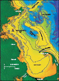Figure 1. Location of long-term mooring at LT-A in western Massachusetts Bay. 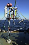Figure 2. Instrumented tripod on deck of USCG Cutter Marcus Hanna. 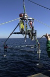Figure 3. Instrumented tripod being deployed from USCG Cutter Marcus Hanna. 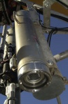Figure 4. Benthos 35-mm underwater camera mounted on tripod. Figure 5. Benthos strobe mounted on tripod frame. The reflector is painted with white antifouling paint to discourage biological growth. Figure 6. Compass and vane assembly mounted in the field of view of the camera. 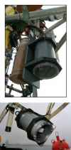Figure 7. New bottom camera (top) and strobe (bottom) mounted on tripod prior to test deployment. 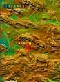Figure 8. Location of tripod moorings (over-lapping red triangles) at LT-A in western Massachusetts Bay deployed from 1989-2005. Table 1. Chronological list of moorings deployed at LT-A in western Massachusetts Bay between 1989 and 2006, and citation for publications. (HTML format; PDF format) 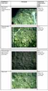Table 5. Identifications of animals and plants observed in the time-series photographs obtained at LT-A.