Woods Hole Science Center
|
Section 3 - Data Collection and ProcessingField program
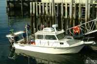
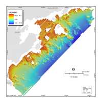
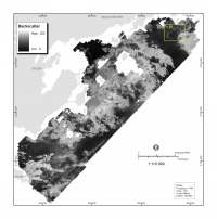
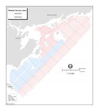
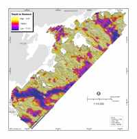
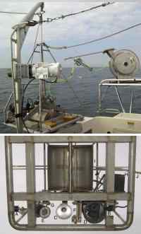
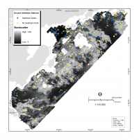
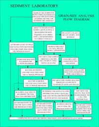
Approximately 134 km² of the inner shelf were mapped using acoustic data from interferometric sonar (bathymetry and backscatter), sidescan sonar (backscatter), and chirp seismic- reflection profiling (stratigraphy and structure). The three systems were simultaneously deployed from the R/V Rafael, a 7.6-m (25-ft) USGS research vessel that is specially outfitted for mapping in nearshore marine, estuarine, and lacustrine, environments (fig. 3.1). Seafloor mapping focused on the nearshore region between the 5 and 40 meter isobaths. Interferometric SonarBathymetry data (water depth) were collected with a SEA Submetrix 2000 series interferometric sonar that operates at a frequency of 234 kHz and configured in a rigid pole-mount on the starboard side of the R/V Rafael. The GPS antenna was mounted on the top of the pole over the sonar head. The system has two channels that collect depth data in a continuous swath on either side of the vessel. The width of the swath is generally 7-10 times the water depth. Under optimal conditions in water depths of 15 m, for example, the interferometric sonar can achieve a 75 m range to each side of the ship's track, or 150 m total swath width. Sidescan SonarAcoustic backscatter data were collected using an Edgetech DF1000 dual frequency (100/500 kHz) sidescan sonar that was towed approximately 25 m astern of the R/V Rafael, and approximately 10 m off the bottom. Backscatter intensity, as recorded with sidescan sonar, is an acoustic measure of roughness of the seafloor (fig. 3.3). Additionally, due to the low angle of incidence of towed systems, topographic highs and lows can be interpreted based on acoustic shadows identified in the imagery. All sonar data were acquired with Triton-Elics ISIS topside acquisition software and later processed for beam angle and slant range correction using LINUX based Xsonar/Showimage as described in Danforth (1997). Sonar data from each survey line were mapped in geographic space in Xsonar and then imported as raw image files to Geomatics GPC works (PCI Geomatica ver 8.2) and mosaiced. The mosaic was exported as a georeferenced tiff image for further analysis in ArcGIS (ESRI Inc). The positional accuracy of the final mosaic is dependant on the estimated towfish layback during acquisition that estimates the horizontal and vertical distance between the GPS receiver and the towfish. Using the Georeferencing toolbar in ArcGIS, the final towed sidescan mosaic was "rubber sheeted" to match the position of the mosaic from the pole-mounted interferometric sonar, which has higher order positional accuracy. Although both the 100 kHz and 500 kHz data were collected, the 100 kHz data were used for the final 1-m mosaic because there was less acoustic noise in the lower frequency data. Seismic-Reflection ProfilingApproximately 1,175 km of high-resolution seismic-reflection profiles (fig. 3.4) were collected using a Knudsen 320b chirp system (3.5-12 kHz). Data were processed using SIOSEIS (Scripps Institute of Oceanography) and Seismic Unix (Colorado School of Mines) to produce segy files and jpg images of the seismic profiles. The segy data were then imported into SeisWorks (Landmark Graphics Inc), an integrated seismic interpretation software package, where selected horizons were digitized to calculate depth to reflections below the seafloor. A constant velocity of 1500 m/s was applied through both water and sediment. Interpreted depth to bedrock (every 5 shots ) was exported into ArcGIS for interpolation into a 50-m grid. Interpreted depth to reflections were calculated, exported every 5 shots, and then imported to ArcGIS for interpolation into a continuous raster with a resolution of 50m/pixel. These data were used to generate a sediment isopach map, which shows the total thickness of sediment between the seafloor and bedrock (fig. 3.5). Ground ValidationThe remotely-sensed data were validated with direct sampling of the surficial sediments and photographs of the seafloor. The ground validation portion of the project commenced immediately following the conclusion of the geophysical surveys in May 2004. One hundred target stations were identified prior to the survey for sampling and photography with the USGS Mini SEABed Observation and Sampling System (Mini SEABOSS; Valentine and others, 2000) (fig. 3.6). Stations were selected based primarily on the previously collected acoustic backscatter data, with the objective of characterizing broad areas of different backscatter intensity (fig. 3.7). In addition, the sampling design included investigation of both gradual and sharp transitions in backscatter values, inferred to be differences in substrates. The research vessel occupied the target location (+/- 10 m), deployed the Mini SEABOSS and drifted with the current over the bottom at approximately 1-3 knots. Continuous video was collected while the camera was within sight of the bottom and photographs were obtained from a still camera at user-selected locations along the transect. Samples of the surficial sediment were usually collected at the end of the drift transect. The upper 2 cm of sediment were scraped from the surface of the grab for textural analysis. At each station about 5 minutes of video and about 5 bottom photographs were obtained. Sediment samples were collected at locations with relatively soft sediment (sand or mud) where the Mini SEABOSS would not be damaged. Samples were not collected in cobble or rocky regions. Samples were analyzed for grain size at the USGS Sediment Laboratory. Poppe and Polloni (2000) describe the standard procedure for grain size textural analysis (fig. 3.8). |
|
![]() To view files in PDF format, download free copy of Adobe Reader.
To view files in PDF format, download free copy of Adobe Reader.
 Back to Maps
 ![]() To Top of Page
To Top of Page  Forward to Next Section