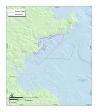
Figure 1.1. Map showing the location of the survey area (outlined in red) offshore of northeastern Massachusetts between Nahant and Gloucester, including part of the South Essex Ocean Sanctuary (blue line).
|
|
Figure 3.1. Photograph of the USGS research vessel Rafael.
|
|
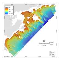
Figure 3.2. Shaded-relief map of seafloor topography offshore of northeastern Massachusetts between Nahant and Gloucester.
|
|
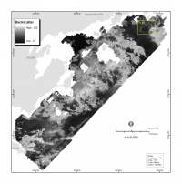
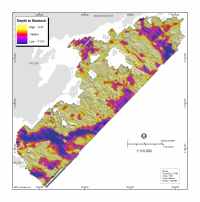
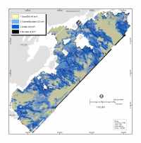
Figure 3.3. Map showing acoustic backscatter intensity offshore of northeastern Massachusetts between Nahant and Gloucester. Backscatter intensity, as recorded with sidescan sonar, is an acoustic measure of the hardness and roughness of the seafloor. In general, higher values (light tones) represent rock, gravel and coarse sand. Lower values (dark tones) generally represent fine sand and muddy sediment. Yellow box (upper right) indicates the location of Figure 4.8.
|
|
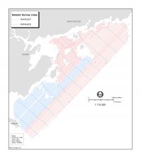
Figure 3.4. Map showing tracklines of seismic-reflection profiles in the survey area.
|
|
Figure 3.5. Isopach map of total sediment thickness in the survey area. Gridded values were interpolated from closely spaced seismic reflection profiles shown in Figure 3.4.
|
|
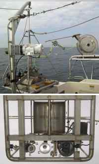
Figure 3.6. TOP: Photograph of Mini SEABOSS and winch on the deck of the RV Rafael. BOTTOM: Components of Mini SEABOSS viewed from below: A) forward video camera; B) downward video camera; C) video light; D) digital still camera and housing; E) strobe light; F) parallel laser for scale; G, laser for ranging; H) junction block; I) van Veen grab sampler; and J) multi-conducting cable.
|
|
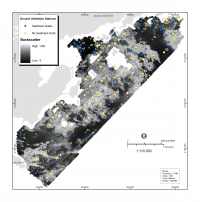
Figure 3.7. Map showing bottom sample locations and video transects overlain on a map of acoustic backscatter from sidescan sonar. Each numbered circle indicates a station where multiple photographs, video, and/or samples were collected.
|
|
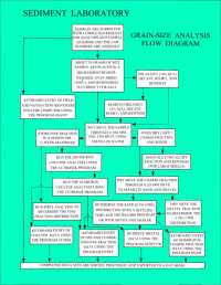
Figure 3.8. Flow diagram showing steps in laboratory analysis of sediment samples (Poppe and Polloni, 2000).
.
|
|
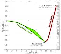
Figure 4.1. Late Quaternary relative sea-level curve for northeastern Massachusetts (modified from Oldale and others, 1993). Over the last 14,500 years, relative sea level fell from a highstand of about +33 m to a lowstand of about -50 m, and then rose at varying rates to the present. These large fluctuations in relative sea level drove regression (red shading) and transgression (green shading) of the shoreline across the inner continental shelf. The dashed lines indicate uncertainty in the sea-level data. Note that the age scale changes at 8,000 years B.P.
|
|
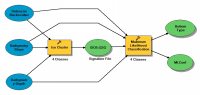
Figure 4.2. Model builder schematic of multivariate analysis, showing input data (depth, slope, acoustic backscatter) and processing steps used to create map in Figure 4.3.
|
|
Figure 4.3. Map of generalized bottom type generated by multivariate analysis of seafloor properties.
|
|
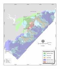
Figure 4.4. Map depicting the physiographic zones of the inner continental shelf. See text for description of zones. Index boxes show locations of inset maps in Figures 4.5, 4.6, 4.7, and 4.8.
|
|
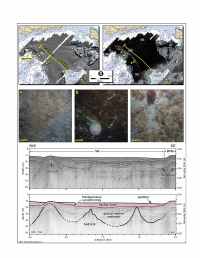
Figure 4.5. Maps of seafloor topography (upper left) and backscatter intensity (upper right) in Salem Sound. Both maps are overlain on NOAA-NOS nautical chart #13275. Dashed lines show boundaries of physiographic zones, which are based on seafloor topography and dominant substrate properties. See Figure 4.4 for location of maps. Bottom photographs A-C (middle) and seismic-reflection profile (bottom) are indicated by yellow circles and line, respectively. The distance across the bottom of the photographs is approximately 50 cm.
|
|
Figure 4.6. Shaded relief map of seafloor topography (upper left) east of Marblehead Neck with red arrows indicating moraine segments. Map of physiographic zones in this area (upper right) is based on seafloor topography and dominant substrate properties. Both maps are overlain on NOAA-NOS nautical chart #13275. See Figure 4.4 for location of maps. Yellow circles indicate bottom photographs A-F (bottom). The distance across the bottom of the photographs is approximately 50 cm.
|
|
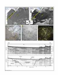
Figure 4.7. Maps of seafloor topography (upper left) and backscatter intensity (upper right) in Nahant Bay and approaches. Both maps are overlain on NOAA-NOS nautical chart #13275. Contour interval is 2 m. See Figure 4.4 for location of maps. Dashed lines show boundaries of physiographic zones, which are based on seafloor topography and dominant substrate properties. Bottom photographs A-C (middle) and seismic-reflection profile (bottom) are indicated by yellow circles and line, respectively. The distance across the bottom of the photographs is approximately 50 cm.
|
|
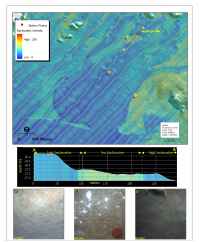
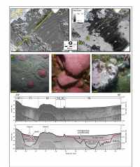
Figure 4.8. Map of seafloor topography colored by backscatter intensity in the northeastern part of the study area. Depth and backscatter data in this map were collected simultaneously by the pole-mounted interferometric sonar, ensuring precise navigation. The depth profile (A - A') crosses a sorted bedform in the upper part of the map; color coding on the profile shows high backscatter material on the floor of a shallow depression. Parallel stripes that trend SW-NE are artefacts of data collection. Bottom photographs B-D are indicated by red circles on map. Map scale is 1:10,000. See figure 3.3 for location.
|
|
Figure 4.9. Maps of seafloor topography (upper left) and backscatter intensity (upper right) in the eastern part of the study area. Both maps are overlain on NOAA-NOS nautical chart #13275. Contour interval is 2 m. See Figure 4.4 for location of maps. Dashed lines show boundaries of physiographic zones, which are based on seafloor topography and dominant substrate properties. Bottom photographs A-C (middle) and seismic-reflection profile (bottom) are indicated by yellow circles and line, respectively. The distance across the bottom of the photographs is approximately 50 cm.
|
|
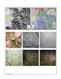
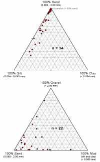
Figure 4.10. Ternary diagrams depicting the texture of surficial sediment collected in grab samples. The apexes of the diagrams represent 100% of the labeled textural component (i.e., gravel, sand, silt, and or clay). The upper diagram depicts 34 samples that lack gravel; the lower diagram depicts 22 samples that contain at least 0.5% gravel. See table 4.2 for additional information on these samples.
|
|
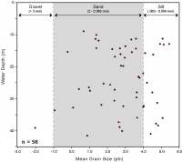
Figure 4.11. Graph depicting the mean grain size versus water depth of sediment samples collected at 56 stations in the survey area.
|
|

 Back to Table of Contents
  Forward to Next Section