 | |
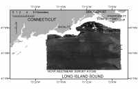
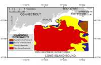
USGS Open-File Report 2005-1162, Sidescan-Sonar Imagery and Surficial Geologic Interpretation of the Sea Floor off Bridgeport, Connecticut
High Backscatter | Low Backscatter | High and Low Backscatter Alternating Bands | Light and Dark Areas | Trawl Marks | Surficial Sediments Distribution | Sedimentary Environments Distribution
|
The sidescan-sonar mosaic of the sea floor off Bridgeport, Connecticut, NOAA survey H11045 (fig. 2), portrays an acoustic image of the sea floor which, combined with subbottom and bathymetric data, can be used to interpret the surficial geology. Distinctive acoustic patterns revealed on the mosaic include:
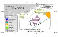
Boundaries between patterns are commonly gradational; backscatter is not uniform throughout these areas. Patchy light and dark areas on the sidescan-sonar image represent dredge spoil disposal mounds. Additionally, several other man-made features appear in the study area. The locations of all features that create distinctive acoustic patterns on the sidescan-sonar image are present in the mosaic interpretation (fig. 6). Locations of the detailed sidescan sonar images discussed throughout this section are shown in fig. 10. Interpretations of the distribution of surficial sediments and sedimentary environments follow the discussion of man-made features. High Backscatter
Areas of high backscatter appear as lighter tones and represent areas of the seafloor characterized by stronger acoustic returns and relatively coarser sediments. The strong acoustic returns are a result of both the geometric effect relating to the angle of incidence of the sand waves and the sand and gravelly sand composition of the sand waves (fig. 7) (Lewis and DiGiacomo-Cohen, 2000). An isolated bathymetric high, southeast of Shoal Point, is composed of sandy sediment. (fig. 7). Low Backscatter
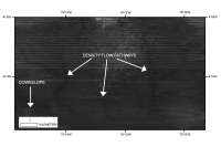
Areas of low backscatter appear as darker tones and represent areas of the seafloor characterized by weaker acoustic returns and relatively finer sediments. The central and southern parts of the study area are characterized by relatively low backscatter, (fig. 2) coinciding with accumulations of fine-grained Holocene marine sediment (fig. 7). Subbottom profiles (Poppe and others, 2002a) show that the deposits of fine-grained sediment thicken southward away from the surface expression of the bedrock. The average thickness of the Holocene marine sediment included in the study area is 5 m. Some of the small isolated spots and patches of higher backscatter that occur within the low-backscatter areas are artifacts of small-scale bathymetric changes that affect the angle of incidence of the sidescan sonar or the result of water column turbulence. Elongate sinuous features of low backscatter that represent sandy silt and clayey silt (fig. 11) range from tens to hundreds of meters wide and can be traced as far as several kilometers. These features extend perpendicular to the bathymetric contours of the Sound and have little, measurable relief. They converge downslope and expand in width. McMullen and others (2005) identified such patterns in their study area as density current pathways, along which remobilized sediments are transported into deeper basins. Alternating Bands of High and Low Backscatter
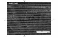
Alternating bands of high and low backscatter characterize parts of the sea floor where sand waves are present. A field of sand waves covers approximately 25 km² of the seafloor in the northeast corner of the H11045 sidescan-sonar mosaic and a smaller field of sand waves off Shoal Point covers approximately 1 km² (fig. 6). The crests of the sand waves in the larger field are oriented north-south and appear as bands of high and moderate to low backscatter (fig. 12). The average wavelength increases from 19 m in the north to 170 m in the south. The 1-km² field of sand waves off Stratford Point, west of the shipping channel into Bridgeport Harbor (fig7.html), are oriented northwest to southeast and have average wavelengths of 23 m. Man-Made FeaturesPatchy Light and Dark Areas
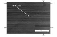
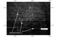
Patches and spots of high backscatter in the center of the image represent dredge spoils (fig. 13). Dredging takes place north of the dumping ground in the ship channel entering Bridgeport Harbor. The high backscatter results from a combination of relatively coarse-grained sediments in dredge spoils or in materials used to cap the spoils, and the angle of incidence of the sonar against the sides of disposal mounds (Morris and others, 1996). Halos of different tones surround some of the disposal piles. These halos may represent the effect of density surges caused by the impact of dredged materials on the bottom or they may represent the subsequent slower sedimentation of the diffuse plume of residual finer-grained spoil material (Schubel and others, 1979). ShipwrecksSeveral shipwrecks are visible, characterized by high backscatter. The weak bottom currents of the western LIS create flow patterns around these wrecks, and linear accumulations of sediment are visible in the acoustic returns. Locations of the wrecks can be found on fig. 6. PipelineA pipeline that was identified in the adjacent NOAA survey H11044 (Mcmullen and others, 2005) is also present in NOAA survey H11045 and is identified by the paired line of high and low backscatter (fig. 14).
Trawl Marks
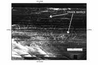
Shallow curvilinear depressions, interpreted to represent trawl marks associated with commercial fishing operations (fig. 15, and fig. 16), occur throughout much of the study area, but are most conspicuous across the northern part (fig. 17). Whether this association is due to an increased visibility of trawl marks within coarser sediments or a preferred biological habitat, is unknown at this time. Some of the trawl marks have a looping appearance. These trawl marks probably owe their extreme curvature to (1) the side-mounted deployment of trawl gear that requires the fishing vessel to turn toward that side to minimize abrasion against the hull, and (2) the practice of trying to stay near an area once a concentration of hard clams has been discovered. Some of the curvilinear depressions, especially the more prominent features, have been labeled as unidentified scars but may be attributed to anchor scars or testing of trawling equipment. Distribution of Surficial Sediments
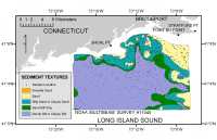
Sandy silt and clayey silt cover the largest area of sea floor in survey H11045 (fig. 7). Aprons of sand-silt-clay separate the coarser material in the northern and eastern portions of the survey from the mud. Sand is present in the north, along the near shore margin of the mosaic and composes the sand waves, formed on top of ice-marginal glaciolacustrine fan deposits, and isolated bathymetric highs identified in the mosaic. Patches of gravelly sand exist in the sand wave field and are identified as the coarsest sediment in the study area. Distribution of Sedimentary Environments
Four sedimentary environments, characterized by erosion or nondeposition, coarse bedload transport, sorting or reworking, and fine grained deposition are mapped within the study area (fig. 8). These environments represent the dominant long-term conditions and may not always reflect small-scale or intermittent processes. For example, erosional bedforms such as sand waves may locally occur in areas characterized by deposition. As with the textural distributions, the contacts between these environments are usually gradational.
Environments characterized by erosion or nondeposition (fig. 18), which reflect high-energy conditions (Knebel and Poppe, 2000; Poppe and others, 2000c), prevail along the relatively shallow waters in the nearshore, northern margin of the study area These environments also exist adjacent to submarine fans along the eastern margin of the image.
The 25-km² field of sand waves in the northeastern corner of the mosaic, and the smaller 1-km² field, represents an environment characterized by coarse bedload transport (fig. 8). The sand waves exist in a convergence zone of potential sand accumulation as modeled by Signell and others (2000). Poppe and Knebel (2000) identified the processes under which sand accumulation in near shore environments is reworked by currents and tides.
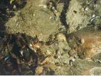
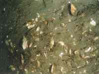
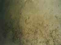
As water depth increases, the strength of storm and tidal currents at the sea floor decreases. Environments that reflect high-energy conditions are replaced by environments of sediment sorting or reworking. Faint current ripples are observed on the surface of grab samples of sandy muds and muddy sands. Sediment resuspension observed in bottom video, reflects this constant sorting by tidal and storm currents. The isolated bathymetric high in the center of the mosaic area is undergoing sediment sorting or reworking. Hermit crabs, starfish, and shell debris are locally common in bottom video observations (fig. 19). The central and southern parts of the study area are characterized predominantly by long-term deposition. In these areas fine-grained sediments accumulate in the deeper, lower energy environments protected from strong tidal and storm conditions. Amphipod and polychaete tubes, shrimp burrows, and snail and rock crab tracks are locally common in these muddy sediments (fig. 20). |