
Two 29-foot launches deployed from the NOAA Ship THOMAS JEFFERSON were used to acquire bathymetric and backscatter data from the study area over approximately 557 km of survey lines during 2004 (fig. 7, fig 8, and fig. 9). The multibeam bathymetric data were collected with hull-mounted 455-kHz Reson 8125 and 240-kHz Reson 8101 systems (fig. 10, and fig. 11). The sidescan sonar data were acquired with a hull-mounted Klein 5250 system operating at 100 kHz (fig. 12). Horizontal resolution of the acoustic data varies with water depth, but averages about 1 m. Vertical resolution is about 0.5% of the water depth.
The survey lines were generally run parallel to the bathymetry contours at a line spacing three to five times the water depth. Navigation was by differential GPS; Hypack MAX was used for acquisition line navigation. Sound-velocity corrections were derived using frequent CTD (conductivity-temperature-depth) profiles (fig. 13). Typically, a CTD cast was conducted every four to six hours of multibeam acquisition. Tidal zone corrections were calculated from data acquired at primary and secondary tide-gauge stations using acoustic stilling-well gauges. Vertical datum is mean lower low water.
The multibeam and sidescan sonar data were acquired in XTF (extended Triton data format), recorded digitally through an ISIS data acquisition system, and processed using CARIS SIPS/HIPS (Sidescan Image Processing System / Hydrographic Image Processing System) software for quality control, to incorporate sound velocity and tidal corrections, and to produce the continuous digital terrain model (DTM) and sidescan sonar mosaic.
A hill-shaded surface was generated from the interpolated grids using ArcGIS 9 with illumination from 315° and from 45° above the horizon. Although choosing a direction parallel to most of the ship's tracks (270°) would minimize artifacts, a direction perpendicular to the ship's tracks was chosen to accentuate geologic features. The geotiff imagery was created with the ArcView Image Conversion Georeferencing extension grid2image and a 5x vertical exaggeration was applied.
Analog high-resolution seismic-reflection subbottom profile boomer data from a previous USGS study (Robb and Oldale, 1977) aided in the geologic interpretation of the multibeam and sidescan sonar data.
To verify the acoustic data, surficial sediments (0-2 cm below the sediment-water interface) and (or) bottom photography were collected at 89 stations (fig. 14) during May-June 2005 aboard the Research Vessel Rafael (fig. 15). The samples and photography were collected with a modified Van Veen grab sampler equipped with still- and video-camera systems (fig. 16). The photographic data were used to appraise intra-station bottom variability, faunal communities, and sedimentary structures (indicative of geological and biological processes) and to observe boulder fields where samples could not be collected. A gallery of photographs collected as part of this project is provided in the Bottom Photographs section of this report.
In the laboratory, the sediment samples were disaggregated and wet sieved to separate the coarse and fine fractions. The fine fraction (less than 62 microns) was analyzed by Coulter Counter; the coarse fraction was analyzed by sieving; and the data were corrected for salt content. Sediment descriptions are based on the nomenclature proposed by Wentworth (1922; fig. 17), the inclusive graphics statistical method of Folk (1974) and the size classifications proposed by Shepard (1954; fig. 18). A detailed discussion of the laboratory methods employed is given in Poppe and others (2005). Because biogenic carbonate shells commonly form in situ, they usually are not considered to be sedimentologically representative of the depositional environment. Therefore, gravel-sized bivalve shells and other biogenic carbonate debris were ignored. The sediment grain-size analysis data can be accessed through the Data Catalog and Sediment Data. sections of this report.
To facilitate interpretations of the distributions of surficial sediment and sedimentary environments, these data were supplemented by sediment data from compilations of earlier studies (Poppe and others, 2003). These other sources include Hathaway (1971), Moore (1963), Hough (1940), and unpublished datasets from the National Geophysical Data Center. The interpretations of sea-floor features, surficial sediment distributions, and sedimentary environments presented herein are based on data from the sediment sampling and bottom photography stations, on tonal changes in backscatter on the imagery, and on the bathymetry. The bathymetric grids and imagery released in this report should not be used for navigation. |
Click on figures for larger images.
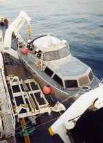 |
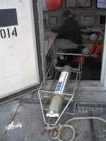
Figure 7. Image showing NOAA Launch 1014 being deployed from the NOAA Ship THOMAS JEFFERSON.
|
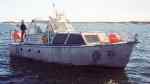 |
Figure 8. Image showing a starboard-side view of NOAA Launch 1014 afloat.
|
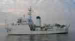 |
Figure 9. Port-side view of the NOAA Ship THOMAS JEFFERSON at sea. Note that the 30-foot survey launch normally stowed on this side of the ship has been deployed.
|
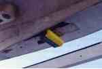 |
Figure 10. Image showing the Reson 8125 multibeam transducer mounted to the hull of the NOAA Launch 1014.
|
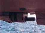 |
Figure 11. Image showing the Reson Seabat 8101 hull mounted in the keel cut out of NOAA Launch 1005.
|
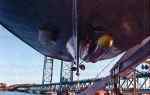 |
Figure 12. Image showing a Klein 5250 sidescan sonar system mounted on the hull of NOAA Launch 1014.
|
 | Figure 13. CTD (conductivity-temperature-depth) profiler shown on the deck of the NOAA ship THOMAS JEFFERSON.
|
 | Figure 14. Map showing the station locations used to verify the acoustic data with bottom sampling and photography during the RAFAEL 05007 cruise.
|
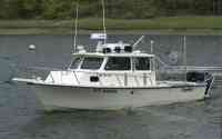 | Figure 15. Image shows a port-side view of the USGS Research Vessel RAFAEL that was used to collect bottom photography and sediment samples in Quicks Hole, Massachusetts.
|
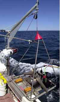 | Figure 16. View of the small SEABOSS, a modified Van Veen grab equipped with still and video photographic systems.
|
 | Figure 17. Correlation chart showing the relationships between phi sizes, millimeter diameters, size classifications (Wentworth, 1922), and ASTM and Tyler sieve sizes.
|
 | Figure 18. Sediment classification scheme from Shepard (1954), as modified by Schlee (1973).
|
|


